The first passage time of a Brownian particle is noise-dependent

Introduction

I noticed that there are conflicting solutions for the expected first passage time of a Brownian particle in the literature. For example, Bogacz, et al. (2006) asserted the expected first passage time is given as

\[ E[t^*] = \frac{b}{\mu}\mathrm{tanh}\left(\frac{\mu b}{\epsilon^2}\right) \]

where \(\mu\), \(\epsilon\), and \(b\) denote the drift, noise term, and boundary, respectively (a more rigorous definition of these parameters is provided below).

On the other hand, according to Wikipedia the first passage time follows an inverse Gaussian distribution with a mean of

\[ E[t^*] = \frac{b}{\mu} \]

Using my own method which I will describe below, I derived that the first passage time follows an inverse Gaussian distribution with a mean of

\[ E[t^*] = \frac{2 b \mu +\epsilon ^2}{2 \mu ^2} \]

My result implies that the first passage time is noise-dependent which I have also verified numerically. Nevertheless, all three solutions have reasonable properties. For example, they all converge to \(\frac{b}{\mu}\) as \(\epsilon \to 0\).

Thus far, no one I have shown these solutions to (including my professor) has been able to identify why our solutions differ. I may eventually devote some effort to reading through the other derivations in detail.

Problem statement

Consider the linear stochastic differential equation

\[ \mathrm{d}x_t = \mu \mathrm{d}t + \epsilon \mathrm{d}W \]

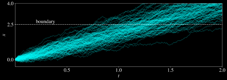
where \(\epsilon\) denotes the strength of the stochastic noise term, \(\mu\) denotes the drift, and \(W\) is a Wiener process. The initial starting point of this equation is \(x_0 = 0\). All parameters (\(\mu\), \(\epsilon\), \(x_0\), and \(b\)) are constant valued and \(b\) and \(\mu \) must have the same sign. The parameter \(b\) represents some boundary that the Brownian trajectories will eventually cross.

The problem is to determine the time step, \( E[t^*] \), at which the Brownian trajectories are expected to cross the boundary, \(b\). \(t^*\) can be expressed as follows

\[ t^* = \inf \left\{ t: \epsilon \int_0^t \mathrm{d}W_t + \mu t \geq b \right\} \]

In the literature, \( E[t^*] \) is often referred to as the expected first passage time.

My solution

From the definition of the Wiener process, it follows that at any time, \(t\), the trajectories follow a Normal distribution with mean \(\mu t\) and standard deviation \(\epsilon \sqrt{t}\). Substituting these values into the Normal cumulative distribution function yields the following expression for the probability of trajectories not having crossed the boundary at \(t\)

\[P(x_t \leq b) = \frac{1}{2}\left[1+\mathrm{erf\left(\frac{b-\mu t}{\epsilon \sqrt{2t}}\right)}\right]\]

Importantly, the cumulative distribution function, \(F(t)\), of the first passage time describes the probability of a given trajectory having crossed the boundary at \(t\). Therefore, \(F(t)\) is simply

\[F(t) = 1 - P(x_t \leq b)\]

The density, \(f(t)\), can be derived by differentiating \(F(t)\) which yields

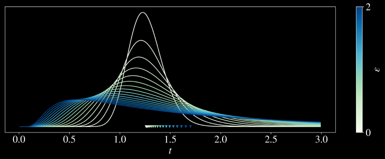
\[f(t) = \frac{\mathrm{d} F(t)}{\mathrm{d} t}=\frac{(b+\mu t) e^{-\frac{(b-\mu t)^2}{2 t \epsilon ^2}}}{2 \sqrt{2 \pi } t^{3/2} \epsilon }\]

Therefore, \( t^* \) follows an inverse Gaussian distribution. This is a rather satisfactory result since it aligns with a plethora of previous research. Moreover, inverse Gaussian distributions are right-skewed as one may also expect for the distribution of \(t^*\). Finally, the expectation of the first passage time can be derived by integration

\[ E[t^*] = \int_0^\infty t f(t)\mathrm{d}t = \frac{2 b \mu +\epsilon ^2}{2 \mu ^2} \]

Thus, the first passage time increases with the level of noise. In the absence of noise, \( E[t^*] \) converges to \(\frac{b}{\mu}\), as expected.

I have also verified this result numerically.